神经网络的计算及paddding为same和valid区别
tensorflow下的程序,很多都是采用padding='SAME',因此如何计算经过卷积操作以后输出层的尺寸,这个时候就要涉及到padding了。
卷积操作以后out=(input+2padding-kernel)/stride+1
*******************************************************************************************************************************
1、关于padding
参考链接:http://blog.sina.com.cn/s/blog_53dd83fd0102x356.html
定义:
Padding在卷积(convolution)和池化(pooling)中都会被用到。在tensorflow比如tf.nn.conv2d,tf.nn.max_pool都有这参数
例子
看例子比较实际:
以一维向量做例子
输入(input)长度:13
过滤器(Filter)长度:6
步长(Stride)长度:5
"VALID" = 不会增加padding:
inputs: 1 2 3 4 5 6 7 8 9 10 11 (12 13)
|_____________| (抛弃不要)
|______________|
"SAME" = 会用0来做padding (如果步长是1的话,最终输出和输入一样大小):
pad| |Pad
inputs: 0| 1 2 3 4 5 6 7 8 9 10 11 12 13 |0 0
|_____________|
|______________|
|_______________|
Notes:
"VALID"会但只会抛弃最右边的列或者是最下面的行."SAME"水平方向首先会在左右各加一个零,如果最后不够的话,会在右边再加零补齐,以满足最后一次完整的移动。对于垂直方向也是同理。
最终输出的行列数计算方法
SAME:
-
out_height = ceil(float(in_height) / float(strides[1]))
out_width = ceil(float(in_width) / float(strides[2]))
VALID:
-
out_height = ceil(float(in_height - filter_height + 1) / float(strides1))
out_width = ceil(float(in_width - filter_width + 1) / float(strides[2]))
因此,当padding=same时,如果stride为1,输入和输出的尺寸是一样的;如果padding=same,stride不为1,(w/s)向上取整
***********************************************************************************************************************
2、举例
①padding=same,stride为1
参考链接:https://blog.csdn.net/zchang81/article/details/67637023
import tensorflow as tf
from tensorflow.examples.tutorials.mnist import input_data


def weight_variable(shape):
    initial = tf.truncated_normal(shape, stddev=0.1)
    return tf.Variable(initial)


def bias_variable(shape):
    initial = tf.constant(0.1, shape=shape)
    return tf.Variable(initial)


def conv2d(x, W):
    return tf.nn.conv2d(x, W, strides=[1, 1, 1, 1], padding='SAME')


def max_pool_2x2(x):
    return tf.nn.max_pool(x, ksize=[1, 2, 2, 1],
                          strides=[1, 2, 2, 1], padding='SAME')


if __name__ == '__main__':
    # 读入数据
    mnist = input_data.read_data_sets("MNIST_data/", one_hot=True)
    # x为训练图像的占位符、y_为训练图像标签的占位符
    x = tf.placeholder(tf.float32, [None, 784])
    y_ = tf.placeholder(tf.float32, [None, 10])

    # 将单张图片从784维向量重新还原为28x28的矩阵图片
    x_image = tf.reshape(x, [-1, 28, 28, 1])

    # 第一层卷积层
    W_conv1 = weight_variable([5, 5, 1, 32])
    b_conv1 = bias_variable([32])
    h_conv1 = tf.nn.relu(conv2d(x_image, W_conv1) + b_conv1)
    h_pool1 = max_pool_2x2(h_conv1)

    # 第二层卷积层
    W_conv2 = weight_variable([5, 5, 32, 64])
    b_conv2 = bias_variable([64])
    h_conv2 = tf.nn.relu(conv2d(h_pool1, W_conv2) + b_conv2)
    h_pool2 = max_pool_2x2(h_conv2)

    # 全连接层,输出为1024维的向量
    W_fc1 = weight_variable([7 * 7 * 64, 1024])
    b_fc1 = bias_variable([1024])
    h_pool2_flat = tf.reshape(h_pool2, [-1, 7 * 7 * 64])
    h_fc1 = tf.nn.relu(tf.matmul(h_pool2_flat, W_fc1) + b_fc1)
    # 使用Dropout,keep_prob是一个占位符,训练时为0.5,测试时为1
    keep_prob = tf.placeholder(tf.float32)
    h_fc1_drop = tf.nn.dropout(h_fc1, keep_prob)

    # 把1024维的向量转换成10维,对应10个类别
    W_fc2 = weight_variable([1024, 10])
    b_fc2 = bias_variable([10])
    y_conv = tf.matmul(h_fc1_drop, W_fc2) + b_fc2

    # 我们不采用先Softmax再计算交叉熵的方法,而是直接用tf.nn.softmax_cross_entropy_with_logits直接计算
    cross_entropy = tf.reduce_mean(
        tf.nn.softmax_cross_entropy_with_logits(labels=y_, logits=y_conv))
    # 同样定义train_step
    train_step = tf.train.AdamOptimizer(1e-4).minimize(cross_entropy)

    # 定义测试的准确率
    correct_prediction = tf.equal(tf.argmax(y_conv, 1), tf.argmax(y_, 1))
    accuracy = tf.reduce_mean(tf.cast(correct_prediction, tf.float32))

    # 创建Session和变量初始化
    sess = tf.InteractiveSession()
    sess.run(tf.global_variables_initializer())

    # 训练20000步
    for i in range(20000):
        batch = mnist.train.next_batch(50)
        # 每100步报告一次在验证集上的准确度
        if i % 100 == 0:
            train_accuracy = accuracy.eval(feed_dict={
                x: batch[0], y_: batch[1], keep_prob: 1.0})
            print("step %d, training accuracy %g" % (i, train_accuracy))
        train_step.run(feed_dict={x: batch[0], y_: batch[1], keep_prob: 0.5})

    # 训练结束后报告在测试集上的准确度
    print("test accuracy %g" % accuracy.eval(feed_dict={
        x: mnist.test.images, y_: mnist.test.labels, keep_prob: 1.0}))
为了方便,我们先定义几个常用的函数:
#使用截断的正太分布,标准差为 0.1 的初始值来初始化权值
def weight_variable ( shape ) :
initial = tf.truncated_normal ( shape, stddev = 0.1 )
return tf.Variable ( initial )
#使用常量 0.1 来初始化偏置 B
def bias_variable ( shape ) :
initial=tf.constant ( 0.1, shape = shape )
return tf.Variable ( initial )
#使用步长 1,填充为 'SAME ' 的方式来初始化卷积层,
def conv2d ( x,w ) :
return tf.nn.conv2d ( x, w, strides = [ 1, 1, 1, 1 ] , padding = 'SAME')
#使用步长为2,下采样核为2 * 2 的方式来初始化池化层,
def max_pool ( x ) :
return tf.nn.max_pool ( x, ksize = [ 1, 2, 2, 1 ], strides = [ 1, 2, 2, 1 ], padding = 'SAME' )
#导入Tensorflow及MNIST数据集:
import tensorflow as tf
from tensorflow.examples.tutorials.mnist import input_data
mnist = input_data.read_data_sets ( "MNIST_data/", one_hot = True )
#定义符号变量 x (数据)和 y_(标签)
x = tf.placeholder ( tf.float32 [ None,784 ] )
y_ = tf.placeholder ( tf.float32, [ None,10 ] )
#先将mnist数据集图片还原为二维向量结构,28 * 28 = 784
x_image = tf.reshape ( x, [ -1, 28, 28, 1 ] )
#第一个卷积层, 总共 32 个 5 * 5 的卷积核,由于使用 'SAME' 填充,因此卷积后的图片尺寸依然是 28 * 28
w_conv1 = weight_variable ( [ 5, 5, 1, 32 ] )
b_conv1 = bias_variable ( [ 32 ] )
b_conv1_1 = conv2d ( x_image, w_conv1 ) + b_conv1
h_conv1 = tf.nn.relu ( conv2d ( x_image, w_conv1 ) + b_conv1 )
#第一个池化层,28 * 28的图片尺寸池化后,变为 14 * 14
h_pool1 = max_pool ( h_conv1 )
#第二个卷积层, 总共 64 个 5 * 5 的卷积核,由于使用 'SAME' 填充,因此卷积后的图片尺寸依然是 14 * 14
w_conv2 = weight_variable ( [ 5, 5, 32, 64 ] )
b_conv2 = bias_variable ( [ 64 ] )
h_conv2 = tf.nn.relu ( conv2d ( h_pool1, w_conv2 ) + b_conv2 )+
#第二个池化层,14 * 14 的图片尺寸池化后,变为 7 * 7
h_pool2 = max_pool ( h_conv2 )
#使用上面定义的方式初始化接下来的两个全连接层的参数 W 和 B
w_fc1 = weight_variable ( [ 7 * 7 * 64, 1024 ] )
b_fc1 = bias_variable ( [ 1024 ] )
w_fc2=weight_variable([1024,10])
b_fc2=bias_variable([10])
#将二维图片结构转化为一维图片结构
h_pool2_flat = tf.reshape ( h_pool2, [ -1, 7 * 7 * 64 ] )
#第一个全连接层,图片尺寸从 7 * 7 * 64 维 变换为1024 维
h_fc1 = tf.nn.relu ( tf.matmul ( h_pool2_flat, w_fc1 ) + b_fc1 )
#第二个全连接层,图片尺寸从 1024 维变换为 10 维的one-hot向量
y = tf.nn.softmax ( tf.matmul ( h_fc1, w_fc2 ) + b_fc2 )
#计算交叉熵loss,并使用自适应动量梯度下降算法优化loss
cross_entropy = -tf.reduce_sum ( y_ * tf.log ( y ) )
train_step = tf.train.AdamOptimizer ( 0.001 ) .minimize ( cross_entropy )
#计算准确率
correct_prediction = tf.equal ( tf.argmax ( y, 1 ) , tf.argmax ( y_, 1 ) )
accuracy = tf.reduce_mean ( tf.cast ( correct_prediction, "float" ) )
#定义一个交互式的session,并初始化所有变量
sess = tf.InteractiveSession ( )
sess.run ( tf.global_variables_initializer ( ) )
#开始训练,测试准确率
for i in range ( 10000 ) :
batch = mnist.train.next_batch ( 50 )
if i % 200 == 0:
train_acc = accuracy.eval ( feed_dict = { x:batch[0], y_:batch[1] } )
print ( "test accuracy", accuracy.eval ( feed_dict = { x:mnist.test.images, y_:mnist.test.labels } ) )
train_step.run ( feed_dict = { x:batch[0], y_:batch[1] } )
②padding=same,stride不为1
参考链接:https://blog.csdn.net/Li_haiyu/article/details/80323962
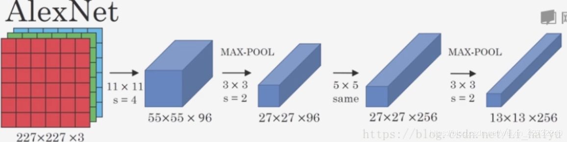
① padding = "value", stride = 4, (227 - 11 + 2*0)/ 4 + 1 = 55
② padding = "value", stride = 2, (55 - 3 + 2*0)/ 2 + 1 = 27
③ padding = "same", stride = 1, 27 / 1 = 27
④ padding = "value",stride = 2, (27 - 3 + 2*0) / 2 + 1 = 13